
Causal Inference: MIT Press Essential Knowledge Series
How Science Distinguishes Real Effects from Mere Association When Randomized Experiments Are Impossible

Chapter-by-Chapter Summaries
Chapter 1: The Effects Caused by Treatments
The opening chapter confronts us with George Washington’s death—not from his sore throat, but likely from his doctors bleeding him based on the ancient theory of humours. This is no mere historical anecdote. It’s the entry point into the fundamental problem of causal inference: to ask whether bleeding caused Washington’s death requires imagining two worlds—one where he was bled (our world, where he died) and one where he wasn’t. We can see only one world. The other remains forever hypothetical.
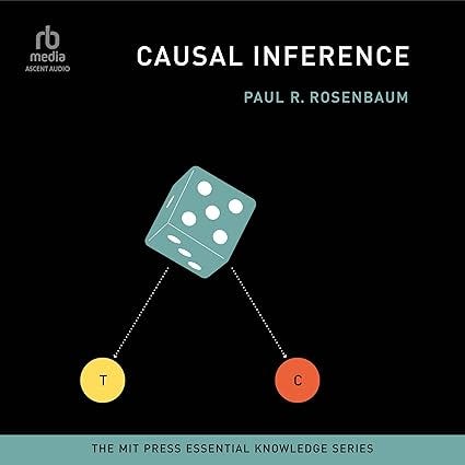
Rosenbaum introduces the notation that will carry through the entire book: lowercase r sub-capital T for the response under treatment, lowercase r sub-capital C for the response under control. The causal effect is their difference—a quantity we can never observe for any single person because that person receives either treatment or control, never both. This is not a limitation of measurement or technology. It’s metaphysical.
The chapter then asks: would a control group solve the problem? Not quite. If Kim survives whether treated or not, and James dies whether treated or not, then comparing treated Kim to control James makes treatment look miraculous (or deadly, depending on the coin flip), when in fact it does nothing. The solution requires something more than just having a control group. That something is randomization.
Chapter 2: Randomized Experiments
The Palm trial in the Democratic Republic of Congo tested two Ebola treatments: ZMapp and mAb114. Of 174 patients receiving mAb114, 64.9% survived 28 days. Of 169 receiving ZMapp, 50.3% survived. This 14.6 percentage point difference could be chance—but the probability of such a difference arising by chance alone if the drugs were equally effective is 0.0083. Seven heads in seven coin flips.
Here Rosenbaum reveals the magic of randomization. It doesn’t make unique people the same—that’s impossible. Washington was unique; any group containing him differs from any group without him. What randomization does is make treatment assignment unrelated to everything that makes people different. Fair coins ignore age, sex, genetic variants not yet discovered, and the potential outcomes that define causal effects.
The chapter walks through Fisher’s insight: randomization balances not just measured covariates (age, sex, blood chemistry) but unmeasured ones too. Those coins knew nothing of the patients’ attributes, so they tended to balance attributes they never saw. More remarkable still: they balanced the potential outcomes themselves—the responses patients would have under each treatment. This makes the difference in observed survival rates between groups a good estimate of the average treatment effect.
The law of large numbers does the rest. With one coin flip for Kim and James, you get the wrong answer whether heads or tails. With 343 coin flips for 343 patients, errors cancel. The casino always wins.
Chapter 3: Observational Studies—The Problem
Daily smokers versus people who never smoked, examined for periodontal disease. Among 1,947 individuals, 441 were daily smokers. If we assigned smoking by fair lottery (22.7% probability), we’d expect roughly equal proportions of men and women to smoke. Instead: 30.4% of men smoked, but only 16.4% of women. The probability of such an imbalance in a fair lottery? 3.2 × 10^-13. In other words: never.
Smokers had less education (29.9% of those without college degrees smoked, versus 7.1% with degrees), less income, and were younger. The estimated probability of smoking ranged from 3.2% (61-year-old college-educated woman, high income) to 64.5% (58-year-old man, less than ninth grade education, income below poverty). A twentyfold difference.
Figure 4 shows smokers have far more extensive periodontal disease than non-smokers—ten times more at the median. But this figure compares people who are not comparable. Perhaps people with more education practice better oral hygiene. Perhaps the pattern reflects decades of brushing and flossing, not smoking. The conspicuous problem—visible differences in measured covariates—can often be fixed. The inconspicuous problem—unmeasured differences in genetics, personality, other addictive behaviors—is harder to address but cannot be eliminated.
Chapter 4: Adjustments for Measured Covariates
Matching creates comparability. Each of the 441 smokers was paired with one of the 1,506 non-smokers who looked similar in terms of age, sex, income, education, and race. After matching, the median age was 47 for both groups, median income nearly identical, median education the same. The nearly tenfold difference in smoking rates between women over 60 with college degrees and men under 60 without college degrees? Gone. Now 50% versus 50.7%.
The propensity score—the probability of smoking given observed covariates—provides one way to think about matching. Before matching, smokers and non-smokers had wildly different propensity scores. After matching, the distributions looked similar. Here’s why this matters: if you pair two people with the same propensity score (say, 0.20), they might be quite different (one a 49-year-old woman with high school degree, the other a 52-year-old man with some college), but those differences won’t help you guess who smokes. The propensity score has already absorbed all the information from age, sex, income, education, and race that predicts smoking.
After matching, smokers still had much more periodontal disease than matched non-smokers. The extensive disease among smokers cannot be explained by differences in age, sex, education, income, or race—because matched non-smokers resembled smokers in these ways yet had much less disease. Could it be something else? Yes. That’s the topic of the next chapter.
Chapter 5: Sensitivity to Unmeasured Covariates
Cornfield and colleagues, writing in 1959 about smoking and lung cancer: “Cigarette smokers have a 9-fold greater risk of developing lung cancer than non-smokers... Any characteristic proposed... must therefore be at least 9-fold more prevalent among cigarette smokers.” No such characteristic had been found. This was the first sensitivity analysis—a quantitative answer to the question: how large would an unmeasured bias have to be to explain away what we see?
For periodontal disease, Rosenbaum quantifies bias using gamma, the maximum odds ratio for treatment assignment within matched pairs. If gamma = 1, we have a randomized experiment. If gamma = 2, one person in a pair might have odds of smoking between 1:2 and 2:1—substantial departure from random assignment. Yet even gamma = 2 is far too small to produce the observed pattern. The probability of such a large effect if gamma = 2 and smoking has no effect on periodontal disease: 0.00018.
A bias of gamma = 2 corresponds to an unmeasured covariate that increases the odds of smoking threefold and increases the odds of periodontal disease fivefold. Even such a covariate wouldn’t begin to explain Figure 8. Compare this to smoking and lung cancer (insensitive to gamma = 5) or seat belt use to prevent death in car crashes (also gamma = 5). Some studies are sensitive to trivial biases (gamma = 1.05) and get contradicted by later randomized trials.
Sensitivity analysis doesn’t provide new data. It supplies quantitative clarification of what’s being asserted by proponents and critics alike.
Chapter 6: Quasi-Experimental Devices in the Design of Observational Studies
Ray and colleagues studied azithromycin (an antibiotic) and cardiac death. They used two control groups: people who received no antibiotic, and people who received amoxicillin (a different antibiotic). Each control group has a flaw. The untreated group likely has fewer infections than those receiving azithromycin—so excess deaths in the azithromycin group might reflect the infection, not the drug. The amoxicillin group also has infections, removing that confound—but if both antibiotics cause cardiac deaths equally, comparing them shows no difference even though azithromycin is harmful.
Together, the two control groups create a design less ambiguous than either alone. Ray found excess cardiac deaths in the azithromycin group compared to both controls. This finding isn’t easily dismissed as caused by infection—after all, the amoxicillin group also had infections.
Eissa and Liebman studied the Earned Income Tax Credit expansion in 1986-1987. Workforce participation among eligible unmarried women without high school degrees rose 1.8 percentage points. But maybe that’s just general economic trends? They examined two “counterpart” groups ineligible for EITC: unmarried women without children (participation fell 2.3 points) and women with college degrees (participation rose 0.9 points). The 1.8 point increase among eligible women isn’t easily dismissed as a general trend—it wasn’t evident in the counterparts.
Quasi-experimental devices strengthen causal claims by undermining specific anticipated counterclaims. They’re not repetition; they’re persistent diligence—adding elements to resolve counterclaims one at a time.
Chapter 7: Natural Experiments, Discontinuities, and Instruments
Jacob and Ludwig studied housing vouchers in Chicago. In 1997, 82,607 eligible applicants were randomized to positions on a waiting list. By 2003, vouchers had been offered to 18,100 families. The offer was randomized—but many people turned down offers. Estimating the effect of the offer is straightforward (offer was randomized). Estimating the effect of receiving a subsidy is harder (accepting wasn’t randomized).
Enter instrumental variables and the complier average causal effect. Some people are “compliers”—they quit smoking only if encouraged, accept vouchers only if offered. We can’t recognize compliers (if Kim quits when encouraged, she might have quit anyway). Yet remarkably, under certain assumptions, we can estimate the average effect for compliers.
The key insight: randomizing encouragement means randomizing quitting for compliers, because compliers do what they’re encouraged to do. Hidden inside a big experiment that randomized the wrong thing is a smaller one that randomized the right thing. Brewer and colleagues found 31% abstinent with mindfulness training versus 6% with standard treatment—25% compliers. If quitting improves lung function, the effect of quitting should be about four times larger than the effect of better encouragement (because most people don’t quit even with better encouragement).
Discontinuity designs find natural experiments at sharp cutoffs. You’re in line for concert tickets. The door slams shut. The last couple to get tickets and the first couple shut out were nearly identical—neither camped out, neither arrived whimsically late. Comparing them is more equitable than comparing campers to latecomers. Near the discontinuity, there’s a natural experiment. Far from it, nothing like random assignment.
Chapter 8: Replication, Resolution, and Evidence Factors
Between 1969 and 2000, three large studies (DARP, TOPS, DATOS) claimed clinical treatment reduces drug addiction. Each claimed to replicate the previous. Yet all three compared people who completed treatment to dropouts—and the National Academy of Sciences noted that dropouts may be more severely addicted or less motivated. “The people who complete their treatment program may be those who are more likely to reduce their drug use, whether or not they receive treatment.”
Seeing the same pattern three times is barely more convincing than seeing it once. For later studies to strengthen evidence, they must eliminate or vary biases that plagued earlier studies.
Contrast this with smoking and lung cancer: heavy smokers showed higher rates; lab studies showed tobacco substances cause cancer in mice; autopsies of smokers revealed precancerous lesions; when women increased smoking (1960s), lung cancer rates rose decades later. Each study is fallible, but many unrelated explanations must conspire to create a false impression that smoking causes lung cancer.
Morton and colleagues studied lead exposure in children of battery factory workers. Three comparisons: workers’ children versus controls (children of workers had more lead); children grouped by father’s exposure level (higher exposure → more lead in child’s blood); high-exposure group split by father’s hygiene (poor hygiene → more lead in child). Each comparison is fallible. But if this doesn’t show an effect, three separate errors are required. The three panels together constitute stronger evidence than any one alone.
Replication is not repetition. It’s removing or varying some potential bias that formed reasonable ground for doubting earlier studies.
Chapter 9: Uncertainty and Complexity in Causal Inference
In 2018, oncologists challenged cardiologists: “The benefit of alcohol consumption on cardiovascular health likely has been overstated. The risk of cancer is increased even with low levels of alcohol consumption, so the net effect of alcohol is harmful.” Cardiologists remain cautious: moderate consumption associates with reduced cardiovascular death and increased HDL cholesterol, but “it should be kept in mind that these are insufficient to prove causality.”
Holmes and colleagues used Mendelian randomization—a genetic variant associated with less drinking. If people received this variant randomly and it affected cardiovascular disease only by reducing alcohol, then the gene is an instrument. They found individuals with the variant had more favorable cardiovascular profiles. “This suggests that reduction of alcohol consumption, even for light to moderate drinkers, is beneficial for cardiovascular health.”
But changing methodology changes the answer from benefit to harm. The answer might be complex—different genes affect alcohol metabolism, cancer risk, heart disease risk differently. Maybe the best advice differs for different people.
The debate concerns the J-shaped curve: does mortality increase steadily with alcohol (no benefit), or does light consumption confer lowest mortality (J-shape)? Both panels show dramatic harm at high levels. What distinguishes them are small effects at low doses—precisely the effects most sensitive to small biases.
Peterson, Trell, and Christensen (1982) found lowest mortality among moderate drinkers, highest among abstainers. But “most of these men... had chronic disease as the reason for their abstention or even a past history of alcoholism.” Some people abstain because they’re ill, not ill because they abstain. The article has not been heavily cited. It says unpleasant truths: appearances deceive, empirical science is difficult, observational studies about small effects can easily give wrong answers.
Does a daily glass of red wine prolong or shorten life? Time will tell. Or maybe not.
Bridge: From Chapters to Synthesis
What emerges from these chapters isn’t a simple story about when observational studies succeed or fail. It’s a portrait of the scientific method as argument—argument conducted in the presence of data, yes, but argument nonetheless. Randomized experiments provide firm ground, but that ground is often inaccessible. We’re left navigating terrain where every claim invites counterclaims, where each study’s weaknesses are different, where resolution comes not from a single decisive experiment but from the accumulation of evidence that eliminates alternative explanations one by one.
The question this book circles—can we know causes without randomization?—never gets a simple yes or no answer. That may be the point. What follows is an attempt to understand what “knowing” means when certainty is impossible, when the best we can do is make some explanations untenable while others remain standing.
Literary Review Essay: The Architecture of Inference When Experiments Are Impossible
When George Washington’s doctors bled him in December 1799, they were not being careless. They were following a theory of disease that had persisted for twenty centuries—the theory of humours, which held that imbalances in bodily fluids caused illness and that restoring balance restored health. They bled him because their teachers believed in bleeding, and those teachers had been taught by teachers who believed, in an unbroken chain reaching back to Hippocrates and Galen. Washington died the next day. Did bleeding kill him?
Paul Rosenbaum’s Causal Inference begins with this question not to answer it (we’ll never know) but to demonstrate why it can’t be answered. To know whether bleeding caused Washington’s death requires seeing two worlds: the one where he was bled and died, and the one where he wasn’t bled and... what? Survived? Died anyway from his sore throat? That alternative world is forever hypothetical. We can stipulate what happens there, but stipulation isn’t observation, and science demands observation.
The entire book unfolds from this dilemma. When you can see only the actual world, how do you learn about possible worlds that never happened? Rosenbaum’s answer proceeds through a kind of methodological archaeology, excavating the tools that twentieth-century science developed to peer into unrealized possibilities. Randomized experiments. Matching on covariates. Sensitivity analyses. Natural experiments and instrumental variables. Quasi-experimental devices that systematically vary the things most likely to mislead us. Each tool addresses some limitation of the one before, and each comes with its own constraints and failure modes.
What makes this a book about inference—that is, about argument and justification—rather than simply about statistical methods, is Rosenbaum’s insistence that counterclaims be taken seriously. An observational study is met with objections, not applause. The common objection says investigators adjusted for measured covariates but failed to control for some unmeasured factor. Philosopher Ludwig Wittgenstein asked: “Doesn’t one need grounds for doubt?” In science, Rosenbaum insists, grounds for doubt are part of the science. A counterclaim must be as rigorous as the claim it challenges. The critic has the responsibility—Rosenbaum quotes Irwin Bross extensively here—”for showing that his counterhypothesis is tenable. In so doing, he operates under the same ground rules as a proponent.”
This creates a particular kind of intellectual drama. The Palm trial, conducted in the Democratic Republic of Congo during an Ebola outbreak, randomly assigned 343 patients to two treatments: ZMapp and mAb114. Of 174 patients receiving mAb114, 64.9% survived 28 days; of 169 receiving ZMapp, 50.3% survived. The 14.6 percentage point difference could be due to chance—an unlucky sequence of coin flips assigning frailer patients to ZMapp—but the probability of such a sequence if the drugs were equally effective turns out to be 0.0083. Not impossible, but improbable enough that maintaining the drugs are equal requires maintaining you observed an extremely unlikely run of bad luck.
Randomization achieves something remarkable: it makes the actual world a random draw from many possible worlds. Certain averages in the actual world then get pulled toward certain averages over possible worlds by the law of large numbers. With one coin flip for two people, you’re a gambler—sometimes you win, sometimes you lose, the answer is always wrong whether heads or tails. With 343 coin flips, you’re a casino. Errors cancel. The average is all there is.
But randomization requires assigning treatments, and that’s often unethical or impossible. You cannot randomize cigarette smoking to study its effects on lung cancer. You cannot randomize emotional trauma to understand PTSD. You cannot randomize minimum wage levels to study their effects on employment. The world gives you observational studies instead—situations where people chose their treatments, or where policies changed for reasons having nothing to do with scientific inquiry.
Rosenbaum’s treatment of smoking and periodontal disease demonstrates the problem. Daily smokers versus never-smokers: 441 compared to 1,506 individuals. If smoking were assigned by fair lottery, you’d expect similar proportions of men and women to smoke. Instead, 30.4% of men smoked but only 16.4% of women. The probability of such an imbalance in a fair lottery? 3.2 × 10^-13. Smokers had less education, less income, were younger. The estimated probability of smoking ranged twentyfold—from 3.2% for a 61-year-old college-educated high-income woman to 64.5% for a 58-year-old man with less than ninth-grade education and income below poverty.
Smokers had ten times more periodontal disease at the median. But this compares people who are not comparable. The solution—matching—creates 441 pairs where each smoker is paired with a non-smoker who resembles them in age, sex, income, education, and race. After matching, smokers still had much more disease. The extensive disease cannot be explained by the measured differences, because matched non-smokers resembled smokers in these ways yet had much less disease.
Could it be something else? Some unmeasured factor? This is where Rosenbaum introduces sensitivity analysis, quantifying how large an unmeasured bias would need to be to explain what we observe. The measure is gamma, the maximum odds ratio for treatment assignment within matched pairs. If gamma equals 1, we have a randomized experiment. If gamma equals 2, one person in a pair might have 2:1 odds of smoking (versus 1:1 in a fair lottery)—substantial departure from random assignment. Yet even gamma = 2 produces the observed pattern with probability only 0.00018. A bias of gamma = 2 corresponds to an unmeasured factor that triples the odds of smoking and quintuples the odds of disease. Even that wouldn’t begin to explain Figure 8.
Compare this to smoking and lung cancer (insensitive to gamma = 5, meaning an unmeasured factor would need to increase odds fivefold) or seat belt use preventing death in crashes (also gamma = 5). Some studies are sensitive to trivial biases (gamma = 1.05) and get contradicted by randomized trials. The point isn’t that insensitivity to bias proves causation—nothing outside a randomized trial does that—but that some claims require increasingly implausible alternative explanations while others collapse at the slightest pressure.
The deepest chapters concern strategies for addressing unmeasured bias through study design rather than post-hoc analysis. Quasi-experimental devices anticipate the most plausible counterclaims and build in additional comparisons that would undermine those counterclaims if the effect is real. Wayne Ray and colleagues studied whether azithromycin increases cardiac death. They used two control groups: people receiving no antibiotic, and people receiving amoxicillin (a different antibiotic). The first control group has a problem—they’re less likely to have infections, so excess deaths in the azithromycin group might reflect the infection rather than the drug. The amoxicillin group also has infections, removing that confound, but if both antibiotics cause deaths equally, the comparison shows no difference even though azithromycin is harmful. Together, the two control groups create less ambiguous evidence. Ray found excess cardiac deaths in the azithromycin group compared to both controls.
Natural experiments seek bits of randomness in an otherwise biased world. Jacob and Ludwig studied housing vouchers in Chicago, where 82,607 eligible applicants were randomized to waiting-list positions. Offers were randomized, but many people declined offers. Estimating the effect of the offer is straightforward. Estimating the effect of receiving a voucher (which requires accepting) is harder because acceptance wasn’t randomized.
This introduces instrumental variables and what Rosenbaum calls the “complier average causal effect”—one of the book’s most elegant results. Some people are “compliers”: they accept vouchers only if offered, quit smoking only if encouraged. We cannot identify compliers (if someone accepts when offered, they might have accepted anyway). Yet under certain assumptions—no one does the opposite of what they’re encouraged to do, and encouragement affects outcomes only by changing behavior—we can estimate the average effect for compliers. The logic: randomizing encouragement means randomizing behavior for compliers, because compliers do what they’re encouraged to do. Hidden inside an experiment that randomized the wrong thing is a smaller experiment that randomized the right thing.
The philosophical weight of the book accumulates around the concept of replication. Between 1969 and 2000, three large studies claimed clinical treatment reduces drug addiction. Each claimed to replicate the previous. Yet all three compared people who completed treatment to those who dropped out—and dropouts may be more severely addicted or less motivated. The National Academy of Sciences noted: “The people who complete their treatment program may be those who are more likely to reduce their drug use, whether or not they receive treatment.” Seeing the same pattern three times is barely more convincing than seeing it once if all three make the same mistake.
Contrast this with smoking and lung cancer, where early studies showed heavy smokers had higher rates, lab studies showed tobacco substances cause cancer in mice, autopsies revealed precancerous lesions in smokers, and when women increased smoking in the 1960s, lung cancer rates rose decades later. Each study is fallible, but many unrelated explanations must conspire to falsely implicate smoking. Replication is not repetition; it’s removing or varying biases that plagued earlier studies.
The final chapter, on alcohol consumption, demonstrates what happens when evidence remains genuinely ambiguous. In 2018, oncologists challenged cardiologists: the benefit of alcohol for cardiovascular health has been overstated, cancer risk increases even at low levels, the net effect is harmful. Cardiologists remain cautious: moderate consumption associates with reduced cardiovascular death and increased HDL cholesterol, but association isn’t causation. Michael Holmes and colleagues used Mendelian randomization—studying a genetic variant that reduces drinking—and found reduced consumption benefits cardiovascular health. But changing methodology changes the answer from benefit to harm.
The debate concerns the J-shaped curve: does mortality increase steadily with alcohol (no benefit), or does light consumption confer lowest mortality? Both panels show dramatic harm at high levels. What distinguishes them are small effects at low doses—precisely the effects most sensitive to small unmeasured biases. Some people abstain because they’re recovering alcoholics, others because medications preclude drinking, others because chronic illness makes it unwise. If these unhealthy abstainers inflate mortality in the abstinent group, light drinking appears beneficial when it isn’t. Peterson, Trell, and Christensen demonstrated this bias in 1982, but the article has not been heavily cited—perhaps because it says unpleasant truths about how easily observational studies mislead.
Does a daily glass of wine prolong or shorten life? Rosenbaum writes: “Time will tell. Or maybe not.”
This is the book’s central insight, delivered with unusual candor. Outside randomized experiments, causal inference is not impossible but it is persistently uncertain. The path of inquiry is “often blocked by intolerance of uncertainty and complexity.” We want simple answers—does X cause Y, yes or no—but for most questions that matter, randomization is infeasible and observational studies give qualified answers that depend on assumptions we cannot fully verify. The best we can do is eliminate explanations one by one until what remains is not certainty but something more modest: diminished grounds for doubt.
What Rosenbaum has assembled is not a toolkit for extracting truth from data but a framework for arguing about causes when the apparatus that normally adjudicates such arguments—the randomized trial—is unavailable. The virtue of this framework is its explicitness about what’s being assumed and what’s at stake. Sensitivity analyses don’t prove robustness; they quantify the magnitude of hidden bias required to overturn conclusions. Quasi-experimental devices don’t eliminate confounding; they make certain confounders untenable by systematically varying them. Natural experiments don’t achieve randomization; they locate situations where treatment assignment approximates a fair lottery.
The result is a book that makes causal inference look harder, not easier—which is a service to science. The eighteenth century believed bleeding patients restored humoral balance for twenty centuries because they lacked what John Dewey called “the experimental habit of mind.” That habit requires acknowledging uncertainty, taking counterclaims seriously, and recognizing that some questions resist the methods we have for answering them. Washington’s doctors had coins, knew how to flip them, could measure outcomes, understood basic probability. What they lacked was the willingness to randomize and observe what happened. We have that willingness now, when ethics and feasibility permit. When they don’t, we have the tools Rosenbaum describes—imperfect tools for navigating terrain where certainty is impossible but inference remains possible.
The question isn’t whether these tools always work. They don’t. The question is what we’re entitled to claim when we use them, and what we’re obligated to acknowledge when their assumptions go unmet. On that question, Causal Inference is uncompromising: we’re entitled to less certainty than we’d like, and obligated to more honesty than feels comfortable. That’s not the message anyone wants from a methodology book. It’s the message science requires.